LAPMOD theory

LAPMOD is a tridimensional and non-stationary Lagrangian particle model that can simulate the atmospheric dispersion of inert or radioactive substances that are emitted as gases or aerosols. Beside conventional pollutants, LAPMOD can simulate the dispersion of odors. The particles used for the calculation move in the atmosphere, driven by mean wind (advection) and turbulence (dispersion). Each particle carries a fraction of the emitted mass. At each instant, it is possible to compute the concentration and the deposition at receptors by considering the position of the particles and their masses.

LAPMOD is implemented in FORTRAN language and it is fully coupled with the diagnostic meteorological model CALMET that provides all the required information about wind speed and direction, and turbulence parameters.

Emissions

LAPMOD allows to simulate the atmospheric dispersion of more substances at the same time, emitted by one or more sources.

The emitted substances can be inert or radioactive, both in gas and aerosol phase. LAPMOD can also simulate the atmospheric dispersion of odors.

The emission rate is always expressed in terms of mass / time (or activity / time or odorimetric units / time), independently from the type of source.

Types of sources

• Point sources with or without thermal buoyancy
• Line sources
• Area sources
• 3D box sources
• Spherical sources
• Polygon sources of arbitrary shape

Releases of radioactive substances

In case of radioactive releases, the emission rates are generally expressed as Bq/s. LAPMOD transforms the activity emission rate in mass emission rate via the specific activity (Knoll, 1979).

Indicating with `A` the activity (in Bq/s), with `M` the molecular wight, with `A_0` the Avogadro number, with `lambda` the decay coefficient (in s) it holds:

`mass = (A M) / (lambda A_0)`

The following relation holds between the decay constant `lamda` and the half-life `T_(1/2)`:

`T_(1/2) = log 2/ lambda`

The conversion factor from the activity rate to the mass emission rate, equal to `M/(lambda A_0)` is a property of the nuclide itself. Obviously, LAPMOD can be used to simulate inert substances as well (that is, non-radioactive). For these substances, the emission rate is already expressed in terms of mass/time.

The transformation of the emission rate from Bq/s to g/s is made in the SETSUB routine.

Gas phase and aerosol phase

The substances released in atmosphere can be gases or aerosols. In case of aerosols, it is necessary to account for the distribution of the sizes of the particles. This distribution is log-normal, with AMAD (Aerodynamic Mean Aerosol Diameter) and GSD (Geometrical Standard Deviation) that depend on the substance and the type of release. The log normal continuous distribution is represented as a discrete distribution in the model, subdividing the interval representing the AMAD in a given number of intervals (NBINS, in general equal to 10) each of them with its probability. For each aerosol particle emitted there are NBINS computational particles generated, each of them with a diameter that equals one of the NBINS intervals.

The number distribution of aerosol particles is log-normal too. The probability to find a particle with diameter less than `l` (that corresponds to the integral of the distribution with `x < l` ) is given by:

`Prob( x < l ) = 0.5 (1+erf(a))`

Where:

`a = (log(l) - log(m)) / (sqrt 2 log (sigma_g))`

and `m` is the geometric mean (that is the median of a log normal distribution) and is the geometric standard deviation.

The volume distribution of particles is proportional to the mass distribution of particles through their (constant) density and it is a log-normal distribution too (Seinfeld and Pandis, 1998, eq 7.51), with the same geometric standard deviation of the number distribution. The median diameter for the volume distribution is given by (Seinfeld and Pandis, 1998, eq. 7.52):

The median diameter for the volume distribution is given by (Seinfeld and Pandis, 1998, eq. 7.52):

`log( mVol ) = log(m) +3log^2(sigma_g)`

Thus, for the volume distribution, the probability to have a volume smaller than is:

`Prob( nu < V ) = 0.5 (1+erf(A))`

Where:

`A = (log(l) - log(mvol)) / (sqrt 2 log (sigma_g)) = (log(l)-log(m)-3log^2(sigma_g)) / (sqrt 2 log (sigma_g))`

The problem is thus finding `A` so that `Prob( nu < V )` is a multiple of (1/NBINS), i.e. to find a value of `A` satisfying:

`erf(A) = 2 Prob( nu < V ) -1 `

Once `A` is known, the corresponding `l` value can be computed via the relation:

`l = exp (A sqrt 2 log( sigma_g ) + log(m) +3log^2(sigma_g))`

Typical AMAD and GSD values for some radionuclides are given by Baklanov and Sorensen (2001), and reported in Table 1.

Nuclide	Half-life (hours)	AMAD (`mu m`)	Deposition velocity (cm/s)	GSD (`mu m`)
Cs-137	2.628E05	0.68	0.1	1.8 - 2.5
Cs-134	1.805E04	0.59	0.12	1.8 - 2.5
I-131	1.930E02	gas / 0.48	0.6	3.0 - 4.0
Te-132	7.820E01	0.81	0.3	1.5 - 2.5
I-133	2.080E01	gas / 0.60	0.7	not available
Ba-140	3.048E02	0.45	0.9	not available
Sr-90	2.549E05	2.50	2	2.0 - 2.5
Ru-103	9.459E02	0.65	0.5	1.4 - 2.5
Pu-238	7.683E05	4.30	2	2.0
Pu-239	2.111E08	4.30	2	2.1
Sr-89	1.212E03	2.50	2	not available

It can be noticed that for the I-131 isotope the gas phase is dominant for the first week after the release.

Meteorological input

The meteorological input of LAPMOD consists of three dimensional fields of wind and temperature and two dimensional fields of turbulent parameters as Monin Obukhov length, friction velocity, convective scale velocity, mixing layer height, etc. LAPMOD can directly read the meteorological fields generated with CALMET (Scire et al., 1999a). CALMET is the diagnostic meteorological model also used in input by the CALPUFF (Scire et al., 1999b) dispersion model that belongs to the list of models suggested by US-EPA. LAPMOD is fully coupled with CALMET.

CALMET is the meteorological model also used for prearing the input to the dispersion model CALPUFF (Scire et al., 1999b). Both CALMET and CALPUFF are available from the Exponent website (http://www.src.com).

CALMET also provides the geophysical variables required by LAPMOD (such as the roughness and the landuse category, used also to estimate deposition fluxes).

LAPMOD can interpolate in time the hourly meteorological output fields of CALMET with frequency specified in input by the user.

Movement of particles within the mixing layer

The trajectory of each particle is given by the sequence of displacements that depend from the local meteorological conditions. It is a first order Markov process; this means that in a mean stationary flow the position of the particles only depends from its position at the previous time step.

The three components of motion are uncorrelated. The displacement in time interval dt depends on the local mean wind and on a random component that evolves according to the Langevin equation:

`d u'_i = a_i(x,u'_i,t) dt + b_(ij) (x,u'_i,t) d xi_j(t) `

`u_i ` represents the mean wind component in the i-th direction and `u'_i` is the turbulent velocity fluctuation in the i-th direction.

The random forcing `d xi` is extracted from a normal distribution with standard deviation equal to `dt`.

The trajectory of each particle is reconstructed through a sequence of displacements with such velocity:

`x_i (t+Delta t) = x_i (t) + Delta t (u_i + u'_i)`

`a` and `b` depend on the local stability conditions that are classified according to the Richardson number `L/z_i` (where `L` is the Monin-Obukov length and `z_i` is the mixing height).

The a coefficient for the vertical component

The `a` coefficient for the vertical component is given by (Franzese et al., 1999):

`a = alpha w^2 + beta w + gamma`

By indicating with `W_n` the n-th moment of the distribution of the vertical velocity fluctuations (that depend on z) and with `GW_n` the corresponding vertical gradient, the `alpha`, `beta` e `gamma` coefficients for unstable conditions (`L/z_i<-1`) are:

`alpha(z) = ( 1/3 GW_4 - 1/2 (W_3) / W_2 (GW_3 - C_0 epsilon) - W_2 GW_2 ) / ( W_4 - W_3^2 / W_2 - W_2^2 ) `

`beta(z) = ( GW_3 - 2 alpha W_3 - C_0 epsilon) / ( 2 W_2 ) `

`gamma(z) = GW_2 - alpha W_2 `

`C_0` is the Kolmogorov constant, equal to 3 according Du (1997), and `epsilon` is the eddy dissipation rate of turbulent energy.

Following Franzese et al. (1999) the second and third moments of the distribution are described by the following analytical expressions:

`W_2 / w_star^2 = a_1 + a_2 (z/z_i)^(2/3) (1- z/z_i)^(4/3)`

`W_3 / w_star^3 = a_3 (z/z_i)(1- z/z_i)^2`

where `a_1` = 0.05, `a_2` = 1.7 and `a_3` = 1.1

The kurtosis is equal to 3.5 (Hibberd and Sawford, 1994), so:

`W_4 = 3.5 (W_2)^2`

And the eddy dissipation rate of turbulent kinetic energy is given by (Luhar and Britter, 1989; Weil, 1990):

`epsilon = 0.4 w_star^3/z_i`

The derivatives of moments respect to z that are present in the `alpha`, `beta` and `gamma` coefficients are obtained by analytically derivating the parameterizations.

For neutral and stable conditions (`L/z_i ge -1`) the `alpha`, `beta` e `gamma` coefficients are:

`alpha(z) = (GW_2)^2 / (2 (W_2)^2) = (GW_2) / W_2 `

`beta(z) = - 1 / T_L `

`gamma(z) = W_2 * GW_2 `

Where `T_L ` is the Lagrangian time scale. Also in this case the derivatives are obtained from the parameterizations.

The a coefficient for the horizontal component

The `a` coefficient for the horizontal component under any stability condition is given by:

`a = - (u'_i) / T_L `

The b coefficient for the vertical component

The `b` coefficient for the vertical component under unstable conditions (L/zi < -1) is given by:

`b = sqrt (C_0 epsilon) `

While for neutral and stable conditions (L/zi ≥ -1) the `b` coefficient is given by:

`b = W_2 sqrt (2/ T_L) `

The b coefficient for the horizontal component

The `b` coefficient for the horizontal component is given, for any stability condition, by:

`b = W_2 sqrt (2/ T_L) `

Turbulence parameterization and Lagrangian time scales

The Lagrangian time scales and the turbulence parameterizations depend on the stability conditions. The hypothesis is that the distribution of particle velocity fluctuations (W2) is the one of the wind velocity fluctuations `W_2 = sigma^2` .

All the equations presented in this paragraph follow the formulation by Hanna et al. (1982), with the exception of the Hurley and Physik (1993) formulation for under convective (i.e. unstable) conditions.

Unstable conditions

Under unstable conditions, the Lagrangian time scales and the velocity fluctuations are computed as:

`T_(Lu) = T_(Lv) = 0.15 z_i/ sigma_v`

`T_(Lw) = 0.6 z_i/ w_star`

`sigma_u = sigma_v`, and `sigma_v` is given by:

`sigma_v = u_star(12-0.5z_i/L)^(1/3) `

Neutral conditions

Under neutral conditions, the Lagrangian time scales and the fluctuation velocities are given by:

`sigma_u = 2 u_star exp (- (3 f z)/(u_star)) `

`sigma_v = sigma_w = 1.3 u_star exp (- (2 f z)/(u_star)) `

`T_(Lu) = T_(Lv) = T_(Lw) = (0.5 z) / (sigma_w (1 +15 (f z)/(u_star))) `

Dove `f` is the Coriolis parameter, `z` is the height above ground and `u_star` is the friction velocity.

Stable conditions

Under stable conditions, the Lagrangian time scales and the fluctuation velocities are given by:

`sigma_u = 2 u_star ( 1 - z / z_i) `

`sigma_v = sigma_w = 1.3 u_star ( 1 - z / z_i) `

`T_(Lu) = 0.15 (z_i / sigma_u) sqrt ( z / z_i) `

`T_(Lv) = 0.07 (z_i / sigma_v) sqrt ( z / z_i) `

`T_(Lw) = 0.10 (z_i / sigma_w) ( z / z_i)^(0.8) `

The motion of particles above mixing height

A particle can reach and go over the mixing boundary layer (BL), because of its motion and because of the possible lowering of the BL when meteorological conditions change.

In such cases, if a particle was within the mixing layer at the previous time step, its fluctuation vertical velocity is set to zero; otherwise no changes are made.

Above the mixing layer the fluctuation velocities of particles evolve according to the Langevin equation for the three components under homogeneous conditions:

`a = - 1 / T_L `

`b = W_2 sqrt (2/ T_L) `

where `T_L` is set to 1000 s and `W_2` to 0.01 m2s-2. It is also assumed that no correlation exists among components.

Particles reflection at ground

When particles reach the ground (i.e. when they are below the roughness length `Z_0`), the particles are perfectly reflected along the vertical according to the relation:

` Z_(n ew) = 2 Z_0 - Z_(old) `

Also the displacement due to the vertical velocity fluctuations is perfectly reflected in the same way.

Effects of thermal buoyancy

Stacks can be considered as being point sources with thermal buoyancy. The plume rise can be estimated in LAPMOD following the approach proposed by Janicke and Janicke (2001) or Webster and Thomson (2005).

Janicke and Janicke algorithm

The Janicke and Janicke (2001) algorithm has the peculiarity to be fit also for plumes with high water content.

The algorithm is three-dimensional and so it can be applied also in situations with highly complex wind fields, and it does not require unrealistic simplifications as wind velocity depending only on vertical elevation and constant direction or even constant wind speed for the whole plume height.

Moreover, the algorithm does not adopt the Boussinesq approximation (i.e. it does not assume that the difference between the plume density and the air density is much smaller than air density), so it can be applied also in situations when the temperature of emission is much higher than air temperature.

For this reason the algorithm is fit for a wide spectrum of source types, from cooling towers, where the emission temperature is only few tens of degrees higher than air temperature, to stacks with scrubbers (e.g. desulphurators) where the temperature of the plume may be some hundreds of degrees higher than air temperature.

The mathematical formulation of the model also allows to simulate a stack with an arbitrary exit direction and to consider both wet (saturated and non-saturated) and dry plumes.

In the following, the main equations of the model by Janicke and Janicke (2001) are presented. The algorithm is solved numerically in LAPMOD, by integrating the equations with a fourth-order Runge-Kutta method.

All the equations of the model are written as a function of distance along the plume axis, denoted with s. The relations between the Cartesian coordinates and the s coordinate are:

` dx / (ds) = u_x / u; dy /(ds) = u_y / u; dz/(ds) = u_z/u`

where `u` is the plume velocity measured along its axis and `u_x`,`u_y` and `u_z` are the Cartesian components of the plume velocity.

The dry air mass conservation equation is:

` (dM) / (ds) = epsilon`

where the mass flux M is given by:

` M = A rho u`

where A is the plume section and `rho` is the plume density. The entrainment coefficient, `epsilon`, can be described in three different ways in LAPMOD.

The conservation of momentum is described by the equation:

` (d(M u_i)) / (ds) = epsilon + delta_(ij) A g (rho_a -rho)`

where "i" iindicates one of the three Cartesian directions (i=1 x, i=2 y, i=3 z) and ` delta_(ij) ` is the Kronecker delta, so the second term in the sum on the right side of the equation is different from zero only for the vertical component. The "a" letter indicates a property of the atmosphere.

The plume water content in vapor phase is described through the specific humidity q, defined as the ratio between the water vapor mass and the total mass of wet air in a given volume. The liquid water content is indicated with ? and it is the ratio between the mass of water in liquid phase and the total mass of wet air in a given volume. The total water content in the plume (vapor phase plus liquid phase) is thus given by ? = ? + q. The equation for mass conservation of water is:

` (d(M xi)) / (ds) = epsilon + xi_a`

The state transition of the water mass in a point of the plume is simulated by computing the saturation value of the specific humidity as a function of temperature in that point of the plume. If the specific vapor content is higher than the saturation value, the exceeding part condensates thus increasing the liquid phase mass.

The equation for the balance of enthalpy is:

` d/(ds) (M(T- h_v/c_p eta)) = -M g/c_p u_z /u rho_a / rho + epsilon (T_a - h_v/c_p eta_a)`

where `h_v` è is the evaporation latent heat and `c_p` is the thermal capacity at constant pressure.

The equations presented are solved numerically after the specification of proper initial conditions. The solutions provide the mean value of the variables of interest on a segment orthogonal to the axis of the plume and for a given value of s. It is assumed that the scalar variables (temperature, water content and possible concentration of any pollutant) have a profile orthogonal to the plume axis as:

`X = X_a + X^star exp (- r^2 / b^2) `

where X is the generic scalar variable, r is the distance from the plume axis and the quantities `X^star` and b satisfy:

`X^star = 3 (X - X_a) `

`b = R / sqrt 3 `

An application of the algorithm to the problem of wet plumes is described in Presotto et al. (2005). In fact, once the average temperature at axis distance s is computed, the profile of temperature is obtained with an equation as the one above, and it is thus possible to compute the specific saturation humidity and the region where the relative humidity of the plume is equal to 100%, i.e. where the condensation takes place. The plume region where the specific liquid water content exceeds a threshold value is the visible portion of the plume.

Regarding the entrainment coefficient, `epsilon`, LAPMOD allows to choose among three different formulations: Janicke and Janicke (2001), Rezacova e Sokol (2000) and Orville et al. (1980).

The entrainment coefficient proposed by Janicke and Janicke (2001) is:

`epsilon = 2 pi rho_a E `

where `rho_a` is the air density (also in the following "a" will denote a property of the atmosphere), and E an entrainment function described as:

`E = lambda R (alpha/2 (w_(per))^2 / w + beta (w_(par))^2 / w + u gamma /(Fr^2))`

where R is the plume radius, `lambda`, `alpha`,`beta`,`gamma`, are empirical coefficients, w è s the modulus of the relative velocity of the plume (wind velocity minus plume velocity), `w_(par)` and `w_(per)` are the components of relative velocity that are parallel and perpendicular to the plume axis, `Fr^2` is the square of the Froude number computed as:

`Fr^2 = (rho u^2) / (abs (rho_a - rho) g R)`

The entrainment coefficient proposed by Rezacova and Sokol (2000) is given by:

`epsilon = (alpha_e T_v) / (R T_(Va)) M`

where `alpha_e` is an empirical coefficient (`alpha_e` = 0.3), R is the plume radius (m), `T_V` is the virtual temperature of the plume (K), `T_(Va)` è is the virtual temperature of the atmosphere (K) and M is the mass flux (kg m‑1 s‑1). By substituting the mass flux expression in the previous equation the following equation is obtained:

`epsilon = pi alpha_e rho u T_v / T_(Va) R`

Orville et al. (1980) adapt a cloud formation model to the description of the plume formed by the emissions of the cooling towers. The entrainment coefficient for a mass of air that raises along the vertical is described by:

`epsilon = (2 alpha) / R M`

with `alpha = 0.075` an empirical parameter equal to 0.075. Substituting M, the previous equation becomes:

`epsilon = 2 alpha pi rho u R`

Webster and Thomson algorithm

The main equations of the model by Webster and Thomson (2002) are presented in the following. The algorithm is solved numerically in LAPMOD by integrating the equations via a Runge-Kutta fourth-order method.

All the equations of the model are written as a function of the distance along the axis of the plume, denoted with s. The relations between Cartesian coordinates and the s coordinate are:

` dx / (ds) = u_x / u; dy /(ds) = u_y / u; dz/(ds) = u_z/u`

where `u` is the plume velocity measured along its axis and ux, uy and uz are the Cartesian components of the plume velocity.

The coupled conservation equations solved by the model are:

` (dF_(m))/(ds) = epsilon`

` (dF_(Mx))/(ds) = -F_m (du_a)/(ds) - D_x`

` (dF_(My))/(ds) = -F_m (dv_a)/(ds) - D_y`

` (dF_(Mz))/(ds) = -F_m (dw_a)/(ds) +B - D_z`

` (dF_H)/(ds) = -F_m c_p (d theta_a)/(ds)`

where ` ul D = (D_x,D_y,D_z)` is the drag force, B is the buoyancy force, ` epsilon` is the entrainment rate of the ambient air mass,` ul (u_a) = (u_a,v_a,w_a)` is the mean wind velocity, ` c_p` is the specific heat at constant pressure. The mass flux ` F_m` , the momentum flux ` ul (F_M) = (F_(Mx),F_(My),F_(Mz))` and the heat flux Fh are given by:

` F_m = pi b^2 rho_p u_s`

` F_(Mi) = (u_(p i) - u_(ai)) F_m`

` F_H = c_p (theta_p - theta_a) F_m`

where ` b=b(t)` is the plume radius, ` u_s` is the modulus of the plume velocity ` ul u_p = (u_p, v_p, w_p)`. Subscripts p and a denote a plume property and an air property, respectively, while subscript i denotes one of the three Cartesian components.

The buoyancy force B and the B and the entrainment rate `epsilon` are computed as:

` B = pi b^2 g (rho_a - rho_p)`

` epsilon = 2 pi b u_e`

where ` u_e` is the entrainment velocity , obtained as:

` u_e = u_e^(rise) + u_e^(turb)`

` u_e^(rise) = alpha_1 abs (Delta u_s) + alpha_2 abs (Delta u_N)`

` u_e^(turb) = alpha_3 min ((epsilon b)^(1/3),alpha_w (1+t/(2 T_L))^(-1/2))`

where, the first component ` u_e^(rise)` is due to the relative motion between the plume and the environment, the second component, `u_e^(turb)` is due to the ambient turbulence, `alpha_1`, `alpha_2` and `alpha_3` are constants, `alpha_w` are vertical velocity fluctuations, `Delta u_s` and ` Delta u_N` are the velocity components relative to the directions parallel and perpendicular to the plume axis, ` T_L` is the Lagrangian time scale.

The three Cartesian components of the drag force are each given by:

` D_i = pi b rho Delta u_s abs (Delta u_N) c_D `

where `c_D ` is the drag coefficient.

The values used for the constants for the plume rise algorithm are typically `alpha_1 = 0.11`, `alpha_2 = 0.5`, `alpha_3 = 0.655` and `c_D = 0.21`. These values can vary and thus they are an input of the LAPMOD model. For example, the entrainment coefficients due to the relative motion between the plume and the environment used by ADMS are `alpha_1 = 0.057` and `alpha_2 = 0.50`. The value `alpha_1` is much different than the values used in other models and in calm conditions it does not allow to estimate a plume rise height that is comparable to the pone obtained with the classical formulas by Briggs or Weil. Instead, the TAPM model uses `alpha_1 = 0.100 ` and `alpha_2 = 0.600`. Typical values of the two entrainment coefficients for the relative motion of the plume are reported in Table 2 (from Webster and Thomson, 2002). For `c_D `, the drag coefficient, there are not many values in literature, so the values previously given are used.

Meteorological conditions	Momentum-dominated rise	Buoyancy-dominated rise
Strong ambient wind (bent over plume). No stratification.	`alpha_2 = 0.35` (Briggs) `alpha_2 = 0.6` (Weil)	`alpha_2 = 0.61` (Briggs) `alpha_2 = 0.6` (Weil)
No ambient wind (vertical plume). No stratification.	`alpha_1 = 0.11` (Briggs)	`alpha_1 = 0.125` (Briggs) `alpha_1 = 0.11` (Weil)
Strong ambient wind (bent over plume). Stratification.	`alpha_2 = 0.6` (Briggs)	`alpha_2 = 0.6` (Briggs)

Turbulence induced by the plume rise

The plume rise effect is to raise the pollutant and enhance the turbulence level inside the plume. The turbulence inside the plume is high close to the release, where temperature and speed are elevated, and it decreases moving away from the point of release due to the entrainment of air with the same characteristics of the surrounding environment.

As already indicated, a computational particle moves in the atmosphere due to the effect of a mean wind and turbulent fluctuations. A particle inside a plume that is rising is instead moved using the velocity components of the plume, computed by LAPMOD using the Janicke and Janicke or Webster and Thomson algorithms, depending on user�s choice. The turbulent fluctuations are in any case summed to them. A random displacement is summed to account for the plume-induced turbulence. The random displacement is extracted from a Gaussian distribution with zero average and V variance, given by (Webster and Thomson, 2002):

`V = (r^2 (t+Delta_t) - r^2(t)) * 0.25`

where r is the plume radius, t indicates the current time and `t+Delta_t` is the time in future. The extent of the displacement is thus large close to the release, when the entrainment activity is maximum and the plume radius grows very quickly, while it reduces moving away from the source, until it is null at the end of the plume rise. Thus, the extent of the displacement reduces along with the reduction of the turbulence induced by the plume. At the end of the plume rise the particles moves due to the mean wind and the turbulent fluctuations caused by the atmospheric effects only.

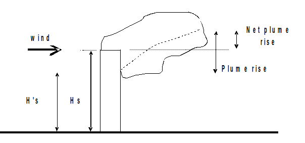
Stack tip downwash

For point source with thermal buoyancy and or mechanical rise, LAPMOD considers also the stack tip downwash (STD).The stack tip downwash phenomenon may happen when the ratio between the exit speed of smokes from the stack and the wind speed at the stack exit is small (i.e. when the wind speed is higher than the exit speed of smokes). In such case, the plume can be captured by the stack wake, resulting in an increase of the concentration values immediately downwind of the stack. This phenomenon is simulated via an algorithm by Briggs that has the practical effect to reduce the physical height of the stack when the conditions generate the STD. When the ratio between stack exit speed (`v_(out)`) and the wind speed at stack exit (`w`) is less than 1.5, the stack height is computed as:

`H'_S = H_S + 2 D ( v_(out) / w - 1.5)`

where `H'_S` is the real stack height and D is its diameter. If instead the ratio of the two speeds is equal or more than 1.5, the stack height remains unchanged (i.e. there is not STD).

Partial plume penetration

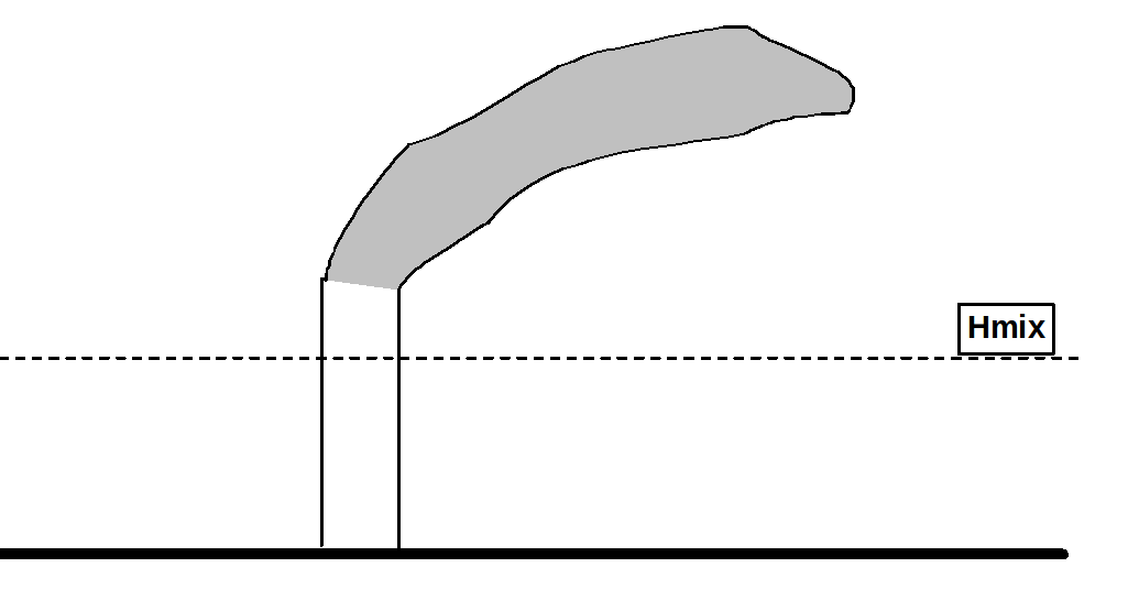
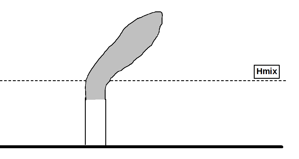
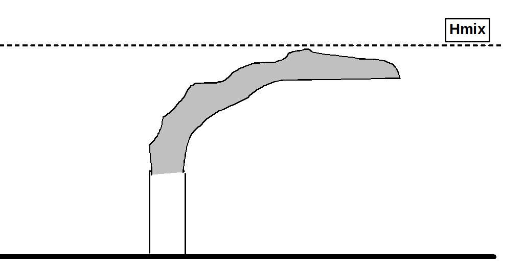
The following sketches show how the plume emitted by a stack may behave depending on the mixing height Hmix. There can be four situations.

	Plume directly emitted above Hmix. This situation is typical of very high stacks under stable conditions when the mixing height is relatively low; this is typical of nighttime. In these conditions the stack top is above Hmix, and the plume is emitted into a layer with limited turbulence so it can stay compact and move as such for relatively large distances.
	Plume emitted below Hmix with enough buoyancy to break Hmix.. Avviene per altezze di rimescolamento non molto elevate e per camini con valori elevati del parametro di galleggiamento, caratterizzati cioè da grandi diametri di emissione, elevate velocità di uscita e temperature di emissione molto elevate rispetto alla temperatura ambiente.
	Plume trapped below Hmix. It happens when the buoyancy parameter is not very large, while there are a high wind speed at stack exit and/or a large difference between the mixing height and the stack height. It also depends on the strength of the thermal elevated inversion (i.e. the temperature difference across Hmix).
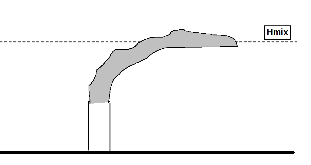
	Plume partially trapped under Hmix. It happens when the buoyancy parameter is comparable to the combined effect of wind speed at stack exit, of the difference between mixing height and stack height and strength of the thermal elevated inversion.

LAPMOD simulates the four conditions described. In particular, the trapping of the plume in presence of an elevated inversion is simulated with the Manins (1979) algorithm, the same used by the CALPUFF model. A penetration parameter, P, is defined as:

` P = (F_b) / (u_s b_i (H_(mix) - H_s))`

where ` u_s` is the wind speed (m/s) at stack height, ` H_s` is the stack height (m), ` H_(mix)` is the mixing height (m), ` b_i` is the strength of the inversion (m/s2) and ` F_b` is the buoyancy parameter (m4/s3). where us is the wind speed (m/s) at stack height, Hs is the stack height (m), Hmix is the mixing height (m), bi is the strength of the inversion (m/s2) and Fb is the buoyancy parameter (m4/s3).

The strength of the inversion is given by:

` b_i = DeltaT / T_(as)`

where ` DeltaT` is the temperature difference across the inversion (K), ` T_(as)` is the atmospheric temperature at stack exit (K), and g is the gravity acceleration. The buoyancy parameter ` F_b` is given by:

` F_b = (g d^2 v_(out) (T_(out) - T_(as)))/ (4 T_(as))`

where ` d` is the stack diameter (m), ` v_(out)` is the emission velocity (m/s) and ` T_(out)` is the emission temperature (K).

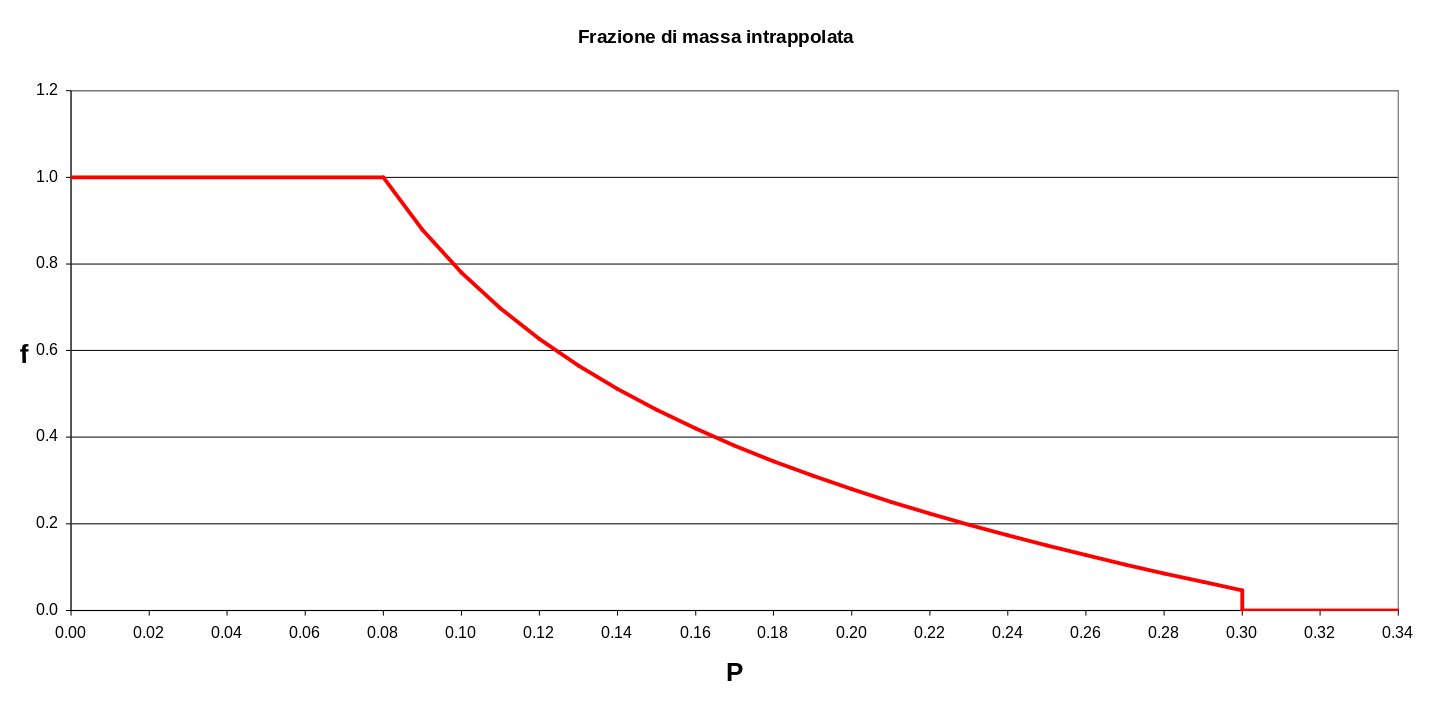
Once the penetration parameter ` P` is known, it is possible to calculate the mass fraction ` f` that remains below ` H_(mix)` . If ` P lt 0.08` , ` f = 1` , then the plume remains completely under the inversion layer; if ` P gt 0.3` , ` f = 0` ,then the whole plume goes above the inversion layer. In all the other cases, when ` 0.08 lt P le 0.3` , the plume mass fraction that remains below Hmix is calculated as:

` f = 0.08 / P - P + 0.08`

The variation of the mass fraction f as function of the penetration parameter P is shown in the next figure.

When ` f > 0` , the final plume rise height is limited by the value:

` z_p = H_s + (1- f/3) (H_(mix) - H_s)`

The penetration parameter (` P` ), the mass fraction below Hmix (` f` ) and the maximum plume rise height (` z_p`) are calculated within the routine PAPLPE. If the result of such a routine is a fraction ` f > 0` , the limitations to buoyancy and plume rise of the particles are imposed within the routine PMOVE.

When the plume is only partially trapped, ` 0 lt f lt 1`, for each particle emitted by the stack a random number (R) within 0 and 1 is generated, and the particle is blocked below Hmix if ` R le f` , otherwise the particle is allowed to go above ` H_(mix)`.

Summarizing, the PAPLPE routine manages the following cases:

` Hs gt Hmix`	The whole plume is emitted above the mixing layer.
` DeltaT = T(z_2) - T(z_1) lt 0`	This is not an inversion, the routine cannot be applied, particles follow the plume rise without any modification.
` Fb lt 0 `	Cold release (release temperature lower then air temperature), the routine cannot be applied, particles follow the plume rise without any modification.
` P gt 0`	Plume completely above Hmix.
` P lt 0.08 `	Plume completely below Hmix.
` 0.08 le P lt 0.3`	The plume goes partially above Hmix. The mass fraction that remains below Hmix is given by f.

Time integration steps

Each computational particle is moved independently from the other ones, and its position is updated up to the moment when concentration and deposition must be calculated. Following Thomson (1987), the condition to apply for determining the time steps for moving the particles along the vertical is:

` Deltat = min(0.05 T_L, 0.1 W_2 / abs(a). 0.01 W_2 / abs (w' GW_2))`

For the horizontal components the time step condition is ?t = 0.15TL, as proposed by the analysis of Wilson and Zhuang (1989) on the errors due to the discretization with different integration intervals in homogeneous conditions.

Moreover, the Courant condition is also applied, so that each particle �feels� the meteorological conditions of all the (meteorological) cells that it has crossed in its path.

Radioactive decay

At each integration time step ` Deltat`, the mass of each computational particle decreases according to the radioactive decay coefficient ` lambda ` of the radionuclide:

` M(t+Deltat) = M(t) exp (-lambda Deltat)`

The radioactive decay is also taken into account for the mass deposited on the ground.

Decay chains are not considered and new species and/or new particles are not generated.

Deposition

A computational particle within the surface layer (assumed equal to 10% of the mixing layer) may lose part of its mass due to dry and wet deposition. This happens both for gases and for aerosols.

In case of dry deposition, the mass lost in a given time step ?t is an exponential function of the deposition velocity, ` v_d`:

` M(t+Deltat) = M(t) exp (-(v_d Deltat)/Z_S)`

where ` Z_S` is the height of the surface layer.

The deposition velocity for gases ` v_d`is obtained by means of the resistances similitude, as for the electric circuits:

` v_d = 1/ (r_a + r_b + r_c) `

The aerodinamic resistence ` r_a` is calculated as suggested by Seinfeld and Pandis (1998):

Stability conditions
Stable atmosphere	` r_a = 1/(k u_(star)) (log(z/z_0) + 4.7 (xi - xi_0))`
Neutral atmosphere	` r_a = 1/(k u_(star) (log(z/z_0))`
Unstable atmosphere	` r_a = 1/(k u_(star)) (log(z/z_0) + log ( ((eta_0^2 +1)(eta_0 + 1)^2) / ((eta_r^2 +1)(eta_r + 1)^2) )) + 2(tan^(-1) eta_r - tan^(-1)i eta_0 ) )`

where ` eta_0 = (1-15 z0/L)^(1/4)`,` eta_r = (1-15 z_r/L)^(1/4)`, `z_0` is the roughness length and `z_r` is the reference height.

The surface resistence is calculated according to Maryon and Ryall (1996):

` r_b = 8 / u_(star)`

The canopy resistencw, ` r_c ` is assumed equal to 500 s/m (Verver and De Leeuw, 1992, Baklanov and Soerensen, 2001).

The dry deposition velocity ` v_d` for aerosols is obtained considering the settling velocity and the algorithms described by Zhang et al. (2001). The settling velocity is calculated using the Stokes law:

` v_(Se t t l) = (rho d^2 g) / (18 eta) C(d) `

where ` v_(S e ttl)` is the settling velocity (m/s), ` r` is the aerosol density (g/m3), ` g` is the acceleration due to gravity (m/s2), ` eta ` is the air viscosity (g/(m s)) and ` C(d)` is the Cunningham correction factor, which depends on the aerosol diameter (determined as explained in Seinfeld and Pandis, 1998).

The aerosol deposition velocity ` v_d` is calculated with the algorithm of Zhang et al. (2001), which increases the settling velocity ` v_(Se t t l)` by a factor depending on the soil occupation category, the friction velocity ` u_(star)` and the season of the year. The soil occupation categories considered in this algorithm are summarized in the following table:

ID	Description
1	Urban
2	Agricultural
3	Range land
4	Deciduous forest
5	Coniferous forest
6	Mixed forest including wetland
7	Water, both salt and fresh
8	Barren land, mostly desert
9	Non forested wetland
10	Mixed agricultural and range land
11	Rocky open areas with low growing shrubs

The dry deposition velocity for gases and aerosols is calculated in LAPMOD within the routine DEPOSD and its subroutines.

The current version of LAPMOD determines the wet deposition only for aerosol species. This is an acceptable approximation because the wet deposition is more effective for aerosols than for gases. The wet deposition velocity is obtained considering both rainout and washout. The efficacy of water droplets in capturing the aerosols depends on several factors:

• the interception of the aerosol from the water droplet,
• the Brownian motion of the particles within the water droplet,
• the enucleation process of a water droplet from a particle,
• the electric attraction,
• the thermal attraction
• the diffusiophoresis

The wet deposition velocity ` v_w` of an aerosol is calculated as described in Baklanov and Sorensen (2001):

` v_w = Lambda H_C`

where ` Lambda` è is the average washout coefficient over the vertical and ` H_C` is the height of the cloud base. The washout coefficient is a function of the aerosol radius and of the precipitation rate, as described by the following equation:

` r lt 1.4 mu m`	` Lambda = a_0 q^(0.79 `
`1.4 mu m lt r lt 10 mu m`	`Lambda = (b_0+b_1 r + b_2 r^2 + b_3 r^3)(a_1 q + a2 q^2)`
`r ge 10 mu m`	`Lambda = a_1 q + a_2 q^2 `

where `a_0`, `a_1`, `a_2`, `b_0`, `b_1`, `b_2`, and `b_3` are constants, `r` is the aerosol radius (`mu m`) and `q` is the precipitation rate (mm/h). For the rainout process the washout coefficient is calculated using the first of the above equations (the one for the small radius).

The wet deposition velocities for aerosols are calculated by the DEPOSW routine and its subroutines.

The mass variation due to the total deposition (dry and wet) in a time interval `Delta_t` can be expressed with the relation:

`M(t+Delta_t) = M(t) exp (- nu Delta_t)`

where ` nu = d + w` is the sum of dry and wet deposition velocity, each one divided by its length.

Dry and wet depositions are two competing processes, but they must be calculated separately to evaluate their contribution to the total deposition. For this reason it is necessary to calculate two equivalent masses ` M_d` and ` M_w` each one subject to one of the two processes:

`M_d(t+Delta_t) = M_(star)(t) exp (- d Delta_t) `

`M_w(t+Delta_t) = M_(star)(t) exp (- w Delta_t) `

Since `M_d(t+Delta_t) = M_d(t+Delta_t) + M_w(t+Delta_t) ` one gets that the equivalent mass (`M_(star)`) that must be used in the two equations above to calculate separately the dry and wet deposition in a time interval `Delta_t` is:

`M_(star)(t) = M(t) (2 - exp(-d Delta_t) -exp(-w Delta_t)) / (1 - exp(-(d+w) Delta_t))`

Concentration

Many Lagrangian particle models calculate the instantaneous concentration at a point (x,y,z) by means of the counting technique, i.e. counting the particles within a specified volume of atmosphere and dividing their total mass by such a volume:

`C_(IST)(x,y,z) = 1 / (Deltax Deltay Deltaz) sum_(i=1)^N m_i`

where:

• `m_i `is the mass of the i-th computational particle for the species of interest,
• `Deltax`, `Deltay` and `Deltaz` (m) are the three dimensions of the volume within which the concentration is calculated,
• N is the number of computational particles within the volume considered.

The counting method is conceptually simple, but it has some disadvantages:

• it requires the generation of a large number of particles, then it increases the simulation times;
• it forces to split the domain in many calculation cells (as for the Eulerian models), and the calculated concentration depends on the cell volume. The gradients of the concentration fields are underestimated if the counting volumes are too large, while discontinuities are present when the volumes are too small.

An alternative approach for calculating the concentrations is the use of a Kernel density estimator.

The term kernel, in the field of Lagrangian particle dispersion models, indicates a mathematical function that allows to calculate the concentration at each point of the space starting from a specific position of the particles.

The concentration at each receptor is calculated as the sum of the contributions of all the particles within the simulation domain. All the particles during their motion are diffused by the atmospheric turbulence, then the masses of two hypothetical particles released at the same time, after some time will be characterized by different spatial distributions, due to the stochastic nature of the diffusive process. Then, with the purpose of calculating the concentration, particles are treated as clouds (distributions) with different sizes and area of influence.

The contribution of a single particle to the concentration at point (x,y,z) at a distance `d_x`, `d_y` and `d_z` from the particle is given by:

`C_i(x,y,z) = (eta m_i)/(2 pi^(3/2) sigma_(x i) sigma_(yi) sigma_(zi)) K_x(d_(x i)/beta_(x i)) K_y(d_(yi)/beta_(yi)) K_z(d_(zi)/beta_(zi))`

where `m_i` is the mass and `sigma_(x i)`, `sigma_(yi)` and `sigma_(zi)`, are the two horizontal and the vertical sigmas of the i-th particle, and `beta_(x i)`, `beta_(yi)` and `beta_(zi)` are scale lengths (the bandwidths). The K functions describe the spatial distribution of the mass associated to the particle and, from a formally point of view, they must only obey to the condition of integrability along the three directions.

LAPMOD incorporates different formulations of the `K` functions.

Gaussian Kernel

The gaussian kernel (Yamada and Bunker, 1988) uses an exponential form for the `K` functions:

`C_i(x,y,z) = (eta m_i)/(2 pi^(3/2) sigma_(hi)^2 sigma_(vi)) exp( -d_(x i)^2/(2 sigma_(hi)^2)) exp( -d_(y i)^2/(2 sigma_(hi)^2)) [exp( -d_(z i)^2/(2 sigma_(vi)^2)) + exp( -d_(z + z i)^2/(2 sigma_(zi)^2))]`

where `m_i` is the mass and `m_i` and `sigma_(hi)` (assuming `sigma_(hi) = sigma_(x i) = sigma_(yi)` ) and `sigma_(vi)` are, respectively, the horizontal and vertical sigmas of the i-th particle; `z_i` is the vertical coordinate of the i-th particle and z is the vertical coordinate of the receptor. The vertical term of the equation also considers the reflection at ground.

The `eta` in the equation guarantees the normalization. Indeed, the contribution of a specific particle to the concentration at a given point is truncated when the distance particle-point exceeds k `sigma` where k is an integer (usually k=3), and for this reason the mass distribution is normalized within the interval `[-k sigma,k sigma]`. In three dimensions the normalization factor `eta` is 1.0081 and it is set to 1 in LAPMOD.

Uniform Kernel

A general expression for the calculation of concentrations at point `(x,y,z)` by means of a kernel is given by Uliasz (1994):

`C_(IST)(x,y,z) = sum_(i=1)^N m_i / (h_(x i) h_(yi) h_(zi)) [K(r_x,r_y,r_z)+K(r_x,r_y,r'_z)] `

where:

• `N` is the number of computational particles contributing to the concentration,
• `m_i` is the mass associated to the i-th computational particle,
• `h_(x i)`,`h_(yi)`,`h_(zi)` are the bandwidths (m) of the i-th computational particle along the three directions.

The bandwidths determine the smoothing degree of the concentration field; they depend on the particle position and on the time.

The non-dimensional distances `r_x`, `r_y` and `r_z` are defined as:

`r_x = (x_i - x) /h_x`

`r_y = (y_i - y) /h_y`

`r_z = (z_i - z) /h_z`

The kernel function K must satisfy the normalization condition:

`1 / (h_x h_y h_z) int_-oo^oo int_-oo^oo int_-oo^oo K dx dy dz = 1`

For the uniform kernel it is defined as:

`K(r_x,r_y,r_z) = alpha_x alpha_y alpha_z I_x I_y I_z`

where `I_i = 1` if `r_i^2 < 1`, otherwise `I_i = 0`. . The bandwidths are defined as proportional to the size of the output horizontal grids (`Deltax, Deltay`) and the the mixing height (Hmix):

`h_x = alpha_x Deltax`

`h_y = alpha_y Deltay`

`h_z = alpha_z H_(mix)`

A typical value for the three multiplicative coefficients is 0.5 (Uliasz, 1994). Those coefficients can be modified within the LAPMOD input file, then the user can evaluate the effect of their values on the calculated concentrations. High values of the multiplication coefficients give a higher smoothing degree to the concentration field, moreover it increases the number of output cells affected by a single particle. Small values of the multiplication coefficients make the bandwidths very small compared with the output cell sizes; in this situations the uniform kernel is very similar to the counting methods.

Parabolic kernel

In the case of the parabolic kernel, the K function is defined as (Uliasz, 1994):

`K(r_x,r_y,r_z) = 15 / (8 pi) (1 - r^2)I`

The bandwidths in x and y direction (`h_x = h_y`) are calculated as in Stohl et al. (1998):

`h_x = A + Bt + C sqrt(t)`

where t is the age of the particle expressed in seconds, A = 20000 m, B = 0.8 m/s and C = 158.771 `m/s^0.5`. The bandwidth along the z direction (`h_z`) is computed with the same expression assuming B=0.

The three bandwidths are limited by independent maximum values (i.e. one for each direction), specified from user input. Typical maximum values are of the order of some few output cells for the horizontal directions (i.e. 1E5m), and comparable to order of magnitude of the mixing height in the vertical direction (from 100 to 1000 m).

Kernel smoother

The kernel smoother is based on the distance between particle and receptor:

`C_i(x,y,z) = { ( m_i /( 4/3 pi sigma_(hi)^2 sigma_(vi)) (1 - d_(x i) / (alpha sigma_(hi))) (1 - d_(y i) / (alpha sigma_(hi))) (1 - d_(z i) / (alpha sigma_(vi))) , if \ d_(ij) le alpha sigma_(ij) \ AA l in {i,j,k} ), (0, otherwise) :}`

where `alpha` is a smoothing parameter that defines the area of influence of a particle.

Both the kernel shape and the smoothing factor are defined by the user through the LAPMOD input file. The smoothing factor may be constant or a function of the particle age.

The sigmas are calculated according to the Batchelor formulation presented by Hanna et al. (1982):

`sigma_(hi)^2 = epsilon t^3` for travel times (i.e. age) of the particle up to `10^4` s and `sigma_(hi) = 100 t` for older particles;

`sigma_(vi)^2 = epsilon t^3` for particle ages up to `10^4` and `sigma_(vi) = 100 t` longer times, but up to a maximum height of `0.3 \ z_i` where `z_i` is the mixing height.

These particle-specific sigmas are calculated at each time step evaluating the local turbulent energy dissipation rate `epsilon`. The total concentration at point (x,y,z) is obtained as the sum of the contributions of all the particles (of course, the sum of the contributions may also be null):

`C(x,y,z) = sum_(i=1)^N C_i(x,y,z)`

where N is the number of computational particles within the simulation domain.

The calculation of concentrations in LAPMOD is carried out within the routine OUTPUT. The concentration values are calculated at each output point - located at the center of each output cell - at the height above the ground specified in the input file.

The output domain of LAPMOD is defined in the input file by means of the coordinates of its LL (lower left) and UR (upper right) corners.

It is also possible to define a list of discrete receptors not belonging to the regular output grid.

The user may also specify the number of sampling between two consecutive outputs of the model. At each sampling the concentration is evaluated, and the output concentration is obtained as the average over all the samplings.

Peak concentrations (odorous, flammable and explosive substances)

The odor impact is usually evaluated in terms of odor concentration expressed as odorimetric unit per cubic meter (OUE/m3), that represents the number of dilution after which the 50% of the odor panelists do not smell the odor from the sample analyzed (UNI EN 13725:2004).

When LAPMOD is used for odor impact studies, the peak concentration, which represents the average concentration over a short period of time (e.g. 5 minutes, 1 minute, or the duration of a single breath, 5 seconds), can be calculated in the classical way by applying the peak-to-mean ratio (PMR) to the 1-hour average concentrations. In this case the PMR is a constant multiplication factor (equal to 2.3 according to the Region Lombardy, Italy, Guidelines of 2012) that is applied during the postprocessing phase with LAPOST (RMULT = 2.3).

In order to make a calculatoin with this simplified approach, it is necessary to make a simulation with any substance and postprocess the results with LAPOST, indicating in input RMULT = 2.3.

The factor 2.3 is an approximation adopted by the Lombardy Guidelines to simplify the calculations. LAPMOD allows to calculate "exactly" the peak-to-mean-ratio according to the original formulation of Smith (1973) and applying the exponential attenuation function of Mylne (1992). Such an approach is also implemented by the Austrian model for atmospheric odor dispersion AODM (Schauberger et al, 2000), and it is described below.

Smith (1973) proposes the following relation for the peak-to-mean ratio:

`Psi_0 = C_p / C_m = ( t_m / t_p)^u`

where `C_m` is the concentration averaged over a long time `t_m`, and `C_p` is the peak concentration over the short time `t_p`. Smith suggests the following values of u, based on the atmospheric stability conditions expressed by the Paquill-Gifford classes:

Stability class	u
A	0.65 (*)
B	0.65
C	0.52
D	0.35
E	0.
F	0.

(*) In LAPMOD, in the case of class-A stability the value for class B is used, since the coefficient for A is not given by Smith (1973).

The choice of `t_p = 5 s`, as short as a breath, is based on the measures of Mylne (1990). These values are strictly valid only close to the source indeed, due to the turbulent mixing, the peak-to-mean ratio decreases after some time from release. In order to describe this effect, Mylne and Mason (1991) derived the following expression for the PMR starting from the analysis of the concentration fluctuations of a plume. The expression includes an exponential attenuation depending from the ratio between flying time T and Lagrangian time:

`Psi = 1 + (Psi_0 -1) \ exp (-0.7317 T / T_L)`

In LAPMOD the atmospheric stability is defined at the release time of the particle and is used to assign to the particle the value of `Psi_0`. The Lagrangian time is calculated as weighted average over the particle movements during the flying time `T = sum_i Delta t_i`, starting on the values encountered by the particle along its trajectory. Such a value is used for calculating the ratio `T / T_L`:

`T/T_L = T^2 / (sum_i (T_{Li} Delta t_i))`

The Lagrangian time can be interpreted as an indicator of the correlation between two consecutive times of the turbulent motion of a particle. Since the Lagrangian time is different for the three spatial components, it is used conservatively the larger value.

The averaging time `t_m` corresponds to the output interval of the concentrations, and the short time `t_p` is an input parameter. In order to apply this calculation method in LAPMOD, it is necessary that the output concentration is an average obtained with more samplings (NSAM > 1).

Since in LAPMOD `t_m` and `t_p` are input variables, the `Psi_0` value is calculated starting from the values of u defined by Smith (1973).

Alternatively, the hourly peak concentration can also be calculated by storing the higher concentration obtained by the samplings used to get the hourly average. For example, if the 1-hour average concentration is calculated with 12 samplings, the higher 5-minute average within each hour will be used.

The LAPOST postprocessor also calculates the FIDOL parameters (Frequency, Intensity, Duration, Offensivity and Location), except offensivity that depends on the odor mixture and has subjective characteristics. The details are reported in the LAPOST user manual.

References

• Baklanov A. and Sorensen J.H. (2001) Parameterisation of radionuclide deposition in atmospheric Long-Range transport modeling. Phys. Chem. Earth (B), Vol. 26, N. 10, pp. 787-799.
• Franzese P., Luhar A.K., Borgas M.S. (1999) An efficient Lagrangian stochastic model of vertical dispersion in the convective boundary layer. Atmospheric Environment, 2337-2345.
• Du S. (1997) Universality of the Lagrangian velocity structure function constant (` C_0`) across different kinds of turbulence. Boundary-layer Meteorology, 83, 207-219.
• Hanna S.R., Briggs G.A. and Hosker R.P. (1982) Handbook on atmospheric diffusion. Technical Information Center, U.S. Department of Energy, pp. 102.
• Hibberd M.F. and B.L. Sawford (1994) A saline laboratory model of the planetary boundary layer. Boundary-layer meteorology, 67, 229-250.
• Hurley P. and Physick W. (1993) A skewed homogeneous Lagrangian particle model for convective conditions. Atmospheric Environment 27A, 619-624.
• Janicke U. and Janicke L. (2001) A three-dimensional plume rise model for dry and wet plumes. Atmospheric Environment, Vol. 35, N. 5, 887-890.
• Knoll G.F. (1979) Radiation, detection and measurement. John Wiley and Sons, Inc. pp. 816.
• Luhar A.K. and Britter R. (1989) A random walk model for dispersion in inhomogeneous turbulence in a convective boundary layer. Atmospheric Environment, 23, 1911-1924.
• Manins P.C. (1979) Partial penetration of an elevated inversion layer by chimney plumes. Atmospheric Environment, 13, 733-741.
• Maryon R.H. and Ryall D.B. (1996) Developments to the UK nuclear accident response model (NAME). Department of Environment, UK Meteorological Office, DoE Report # DOE/RAS/96.011.
• Mylne K.R. (1990) Concentration fluctuation measurements in a dispersing at a range up to 1000m, Q.J.R Meteorol. Soc., 117, 177-206.
• Mylne K.R. (1992) Concentration fluctuation measurements in a plume dispersing in a stable surface layer. Boundary-layer Meteorology, 60, 15-48.
• Mylne K.R. and Mason P.J. (1991) Concentration fluctuation measurements in a dispersing at a range up to 1000m, Q.J.R Meteorol. Soc., 117, 177-206.
• Orville H.D., Hirsch J.H. and May L.E. (1980) Application of a cloud model to cooling tower plumes and clouds. Journal of Applied Meteorology, Vol. 19, 1260-1272.
• Presotto L., R.Bellasio and R.Bianconi (2005) Assessment of the visibility impact of a plume emitted by a desulphuration plant. Atmospheric Environment, 39(4), 719-737.
• Rezacova D. and Sokol S. (2000) On the influence of cooling towers on weather and climate. Czech Hydrometeorological Institute, 77 pages.
• Scire J.S., Robe F.R., Fernau M.E. and Yamartino R.J. (1999a) A user's guide for the CALMET meteorological model (Version 5.0). Earth Tech Inc., September 1999.
• Scire J.S., Strimaitis D.G., and Yamartino R.J. (1999b) A user's guide for the CALPUFF dispersion model (Version 5.0). Earth Tech Inc., May 1999.
• Seinfeld J.H. and S.N. Pandis (1998) Atmospheric chemistry and physics. From air pollution to climate change, John Wiley & Sons.
• Shauberger G., M. Piringer and E. Pets (2000) Diurnal and annual variation of the sensation distance of odour emitted by livestock buildings calculated by the Austrian odour dispersion model (AODM). Atmospheric Environment, 34, 4839-4851.
• Smith M.E. (1973) Recommended Guide for the Prediction of the Dispersion of Airborne Effluents. ASME, New York.
• Thomson D.J. (1987) Criteria for the selection of stochastic models of particle trajectory in turbulence flows. J.Fluid Mech., 180, 529-556.
• Uliasz, M. (1994) Lagrangian particle dispersion modeling in mesoscale applications, in: Environmental Modeling, Vol. II, edited by: Zannetti, P., Computational Mechanics Publications, Southampton, UK.
• Verver G and F.A.De Leeuw (1992) An operational puff dispersion model. Atmospheric Environment, 26,17,3179-3193.
• Webster H.N. and Thomson D.J (2002) Validation of a Lagrangian model plume rise scheme using the Kincaid data set. Atmospheric Environment, Vol. 36, N. 32, pp. 5031-5042.
• Weil J. C. (1990) A diagnosis of the asymmetry in top down and bottom up diffusion using a Lagrangian stochastic model. Journal of Atmospheric Science, 47, 501-515.
• Yamada T. and Bunker S. (1988) Development of a nested grid, second moment turbulence closure model and application to the 1982 ASCOT Brush Creek data simulation. Journal of Applied Meteorology, 27, 562-578.
• Zhang L., Gong S., Padro J. and Barrie L. (2001) A size segregated particle dry deposition scheme for an atmospheric aerosol module. Atmospheric Environment, 35, 549-560.