Modelling industrial flares impacts
Abstract
This document introduces a new software to estimate the atmospheric impact of industrial flares. The software allows to design stacks with correct height and diameter in order to minimise risks for workers and nearby structures. It also allows to estimate the thermal impact and acoustic impact of existing or future flares. Flame tilting due to the wind speed can be modelled with a simple methodology and with the Brzustowski and Sommer (B&S) approach. The software also determines the flue gas composition starting from the fuel gas composition. The effective source parameters to be used as input in atmospheric dispersion models are determined with two different methods: US EPA SCREEN3 and TCEQ.
A PDF version of this document is available from this link.
Software availability
The FLARES software described herein has been developed by Enviroware srl in Visual Basic using the .NET framework. It works under any recent Windows operating system. It can be evaluated at no cost for a limited time period. The permanent license of the software is bound to a single PC, and can be purchased from the web site or directly from the software.
Read more and try FLARES for free
1. Introduction
The majority of chemical plants and refineries have flare systems designed to relieve emergency process upsets that require release of large volumes of gas via flaring or venting operations. Flaring operations are the controlled burning of gases, in open flames and open air, in the course of routine oil and gas production. Venting, on the contrary, is the controlled release of gases into the atmosphere, without combustion.
The gas combustion usually occurs at the top of a flare stack which is placed in a remote site of the plant. Flare systems have been technically described in many papers (e.g. Bader et al. 2011; Hong et al. 2006).
When a flare operates, it generates noise, heat radiation, and emits atmospheric pollutants. If the combustion is efficient, which means to have a good mixing between the fuel gas and air, the emitted gases are mainly water vapour and carbon dioxide. Even if the combustion efficiency may be higher than 90%, other pollutants are generally present, such as carbon monoxide (CO), nitrogen oxides (NOX), sulphur dioxide (SO2), volatile organic compounds (VOC) and particulate matter (PM). VOCs derive by incomplete combustion of the flared gas, or by its conversion to other compounds, such as aldehydes or acids. However, VOC elimination is nearly complete, exceeding the 98%. Concerning smoke formation, it is most probable in streams with high carbon/hydrogen mole ratio (greater than 0.35). Some regions of the world are heavily affected by flares pollution (Obia et al., 2011).
Industries would have all the advantages to avoid flaring, however such operation is necessary under different circumstances as, for example:
- to release high pressure in the plant and avoid catastrophic situations;
- after process upsets, equipment changeover or maintenance;
- to burn vapours collected from the tops of tanks as they are being filled;
- to release unburned process gas from the processing facilities;
- to eliminate the excess gas which cannot be supplied to customers.
Both elevated and ground level flares exist. They can also be classified according to the method used for enhancing mixing between air and fuel. In the steam-assisted flares steam is injected into the combustion zone to promote turbulence and entrain air into the flame. In the air-assisted flares forced air is used to provide the combustion air and mixing; these flares can be used when steam is not available. The non-assisted flares do not have any mechanism for enhancing the air-flame mixing; they are used for gases with a low heat content and a low carbon/hydrogen ratio (such ratio is related to the smoke production). Finally, the pressure-assisted flares use the vent stream pressure to promote mixing between air and flame.
This document describes the structure and some example applications of a software specifically developed to correctly design the stack of subsonic flares, evaluate the heat radiation and noise levels of subsonic or sonic flares, and determine the flue gas composition and the effective stack parameters for atmospheric dispersion applications.
Software description
Theory
The calculations implemented into the software are mainly based on the methodology described in the ANSI/API Standard 521, fifth edition January 2007 (API, 2007), and on the US-EPA technical documentation (EPA, 1995).
The radiation level K (kW/m2) at distance d (m) is calculated, assuming the flame as a single radiant point located at its centre, using the following equation:
`K = (tau F Q ) / (4 pi d^2)`where F is the fraction of heat released which is radiated (-), Q is the heat liberated (kW) obtained multiplying the mass flow rate (kg/h) by the heat of combustion (kJ/kg), and t is the transmissivity (-), which is the fraction of heat radiated transmitted through the atmosphere.
The transmissivity depends on how atmosphere absorbs the radiated heat. Since water vapour is the most important absorber in air, relative humidity will play an important role. In fact, an empirical equation to calculate transmissivity is (Brzuwstoski and Sommer, 1973):
`tau = 0.79 (3000 / (R H d))^(1/16)`where RH is the relative humidity (%).
A graphical empirical relation allows to relate the heat liberated by the flame to its length. Such graphical relation, and others, have been digitised within the software. Flame tilting due to the wind can be calculated either with a simple method which relates the horizontal and vertical displacement of the flame centre with the ratio between wind speed and gas exit speed, or with the Brzuwstoski and Sommer (1973) approach which depends on the lower explosive limit concentration of the flared gas and on the jet thrust and wind thrust parameters. Once determined the flame length and its tilting, the position of the radiant point is placed half way between the flare tip and the flame tip.
The stack height and diameter can be calculated in two different ways according to the user choice:
- by specifying an allowable radiation at an horizontal distance from the stack base (point B in Figure 1) or
- by specifying an allowable radiation directly under the flame centre (point A in Figure 1).
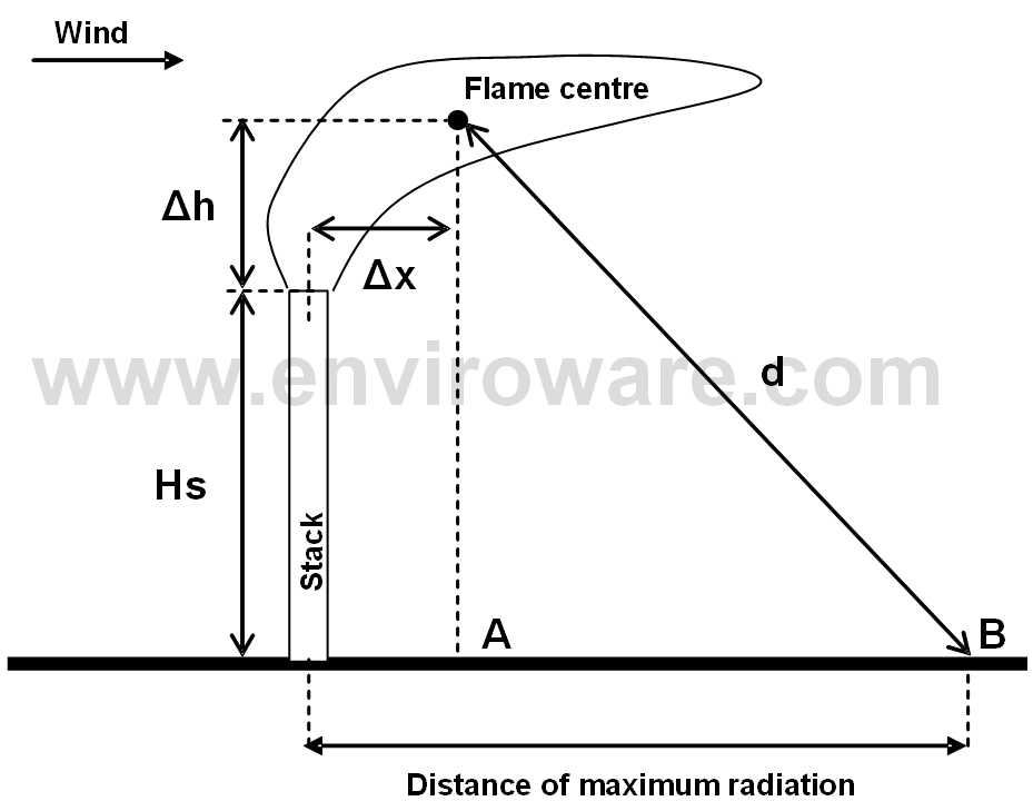
The distance from the flame centre to the point of interest (A or B) is calculated by inverting equation (1) and assuming a constant unitary transmissivity. If the constrain for determining the stack height is the maximum radiation allowed directly under the flame centre, once calculated the distance d, the stack height is obtained by subtracting the displacement of the flame centre from the stack tip height, which is known. If the constrain is the allowable radiation at a specific horizontal distance from the stack base, the stack height is obtained by applying the Pythagoras� theorem (the displacement of the flame centre from the stack tip, ?h and ?x, are known after the tilting calculation).
The stack diameter is determined by inverting the equation for the Mach number, which is an input value, and which depends on the mass flow rate, the relative molecular mass of the flare gas, the flowing temperature, the absolute temperature within the flare tip and the compressibility factor.
Once the theorethical stack height and diameter have been calculated with the above procedure, their actual values must be chosen on the market from those just greater than the calculated values.
Equations (1) and (2) are used for determining the heat radiation levels at specific horizontal distances from the stack base and at specific heights above the ground.
The noise levels are calculated as explained in API (2007). Initially the noise level at 30 m is calculated starting from the mass flow (kg/h), the speed of sound in the gas (m/s), and the pressure ratio, which is the ratio between the static pressure upstream from the restriction and the absolute pressure downstream of the restriction. At distances greater than 30 m the noise level decays in a way proportional to the logarithm of the distance.
The flue gas parameters are determined starting from the stream composition expressed in percent of volume, the mass flow rate and the excess of air, and applying stoichiometry. Starting from these data the methodology initially calculates the gas stream parameters (molar weight, normal density, volume and mass flow rate, heat released, and moles of C, H, O, N and S), then the flue gas parameters are determined (molar weight, mass and volume flow rate, normal density, water content, oxygen content in dry flue gas, dry volume flow rate, concentration of pollutants and emission rates of pollutants). The emission rate of SO2 is calculated starting from the sulphur contained within the fuel gas stream. The emission rates of the other pollutants (NOX, CO, VOC and PM) are calculated using the AP42 emission factors. The VOC emission rate can be alternatively calculated indicating a destruction efficiency. For example, if the destruction efficiency is 98%, the 2% of the VOCs within the fuel gas stream will be emitted into the atmosphere.
The effective stack parameters which must be used within the atmospheric dispersion models (e.g. AERMOD, CALPUFF) are calculated using two different methods: the US EPA SCREEN3 (EPA, 1995) method, and the TCEQ (Texas Commission on Environmental Quality) (TCEQ, 2004) method. The main difference between the two methods is that the TCEQ method does not consider an additional plume height for the length of the flame. Both the two methods equate the buoyancy flux calculated by the Briggs (1969) equation with the buoyancy flux calculated starting from the actual buoyancy of the flare combustion gases.
`g nu d^2 (T - T_a) / (4T) = 3.7 xx 10^(-5) Q_h`where `Q_h` is the sensible heat obtained as `Q_h = FQ`, expressed in cal/s, which is known. Assuming specific values for the stack temperature T (K), the air temperature Ta (K) and the stack exit velocity v (m/s), by inverting the equation, it is possible to obtain a value for the equivalent diameter dE (m) as
`d_E = 3.7 xx 10^(-5) (4 T Q_h) / ((T-T_a) g nu`The stack temperature T is often assumed to be 1273 K, while the ambient temperature Ta and the stack exit velocity v depend on the specific location. The exit velocity v must be chosen to avoid the stack tip downwash, therefore v > 1.5 u, where u is the wind speed. If v = 20 m/s and Ta = 293 K, a simplified form of the above equation is
`d_E = 9.90 xx 10^(-4) (Q_h)^(1/2)`With the TCEQ method the fraction of heat radiated F is calculated by means of the Tan (1967) expression: F = 0.048 M0.5, where M is the molar weight of the gas stream. On the contrary, with the SCREEN3 EPA method F is usually assumed equal to 0.55.
Using the TCEQ method, the equivalent diameter, the exit speed and the exit temperature are used for calculating the plume rise, and the effective release heigth of the plume is obtained by the sum of the flare stack height and the plume rise height. No additional height for the length of the flame is considered, therefore the user will insert in the atmospheric dispersion model the equivalent diameter, the exit velocity (e.g. 20 m/s), the exit temperature (e.g. 1273 K), and the flare stack height, together with the emission rates of the pollutants.
It is observed that for complete combustion of hydrocarbons the temperature of the flare flame should be 1200 K (Attar et al., 2007), which is also the temperature at which NOX begins to form.
With the EPA SCREEN3 method, an equivalent stack height `Q_E` is calculated by adding to the stack the flame length, assuming a tilt of 45 degrees:
`h_E = h_S 4.56 xx 10^(-3) (Q)^(0.478)`where `h_S` is the flare stack height and Q is the total heat release (cal/s). When this method is adopted, the user will insert in the atmospheric dispersion model the equivalente diameter, the equivalent stack height, the exit velocity (e.g. 20 m/s), the exit temperature (e.g. 1273 K), together with the emission rates of the pollutants.
2.2 Features
FLARES is a Windows application written in Visual Basic using the .NET framework. A brief list of the main features of the software are:
- Ability to size (i.e. to calculate the minimum values of height and diameter) subsonic industrial flares according to a specified allowable radiation;
- Calculation of thermal radiation and noise levels of subsonic and sonic flares;
- Flame tilting calculated with the Simple approach and with the Brzustowski and Sommer approach;
- Calculation of the flue gas composition starting from the fuel gas composition;
- Calculation of the effective stack parameters needed for dispersion modelling;
- Ability to works with SI (International Standard) and USC (United States Customary) units;
- Load and georeferentiate raster base maps (automatic georeferentiation if the base map file has an associated world file);
- Position the stack over the base map;
- Thermal radiation levels and noise levels are shown at any point moving the mouse over the base map;
- Plots radiation levels and noise levels over the base map;
- Stack can be exported in KML format for Google Earth as a 3D cylinder;
- Thermal radiation levels and noise levels can be exported in KML format for Google Earth.
Flue gas composition and atmospheric dispersion
Mass flow rate and stream composition allow to calculate flue gas parameters, among which the heat liberated by the flame and the molar weight, and the flue gas parameters. The net heat release can be used for verifying if the flare will meet the minimum heating value requirements of 40 CFR � 60.18.
Starting from the stream composition indicated in Table 1 the values indicated by Alizadeh-Attar et al. (2007) are used as an example and using a mass flow rate of 10000 kg/h, an excess of air equal to 250%, a reference oxygen value equal to 3%, and a molar weight of the air equal to 28.85, the output stream composition reported in Table 2 is obtained. Remembering that 1 Btu corresponds to 0.293 Wh, and 1 Nm3 corresponds to 37.326 scf, dividing the total heat released of 578520 kW by the volume flow rate of 47559.2 Nm3/h, and transforming the units, a heating value of 1112.3 Btu/scf is obtained, which compares very well with the value of 1111.5 Btu/scf observed by Attar et al. (2007).
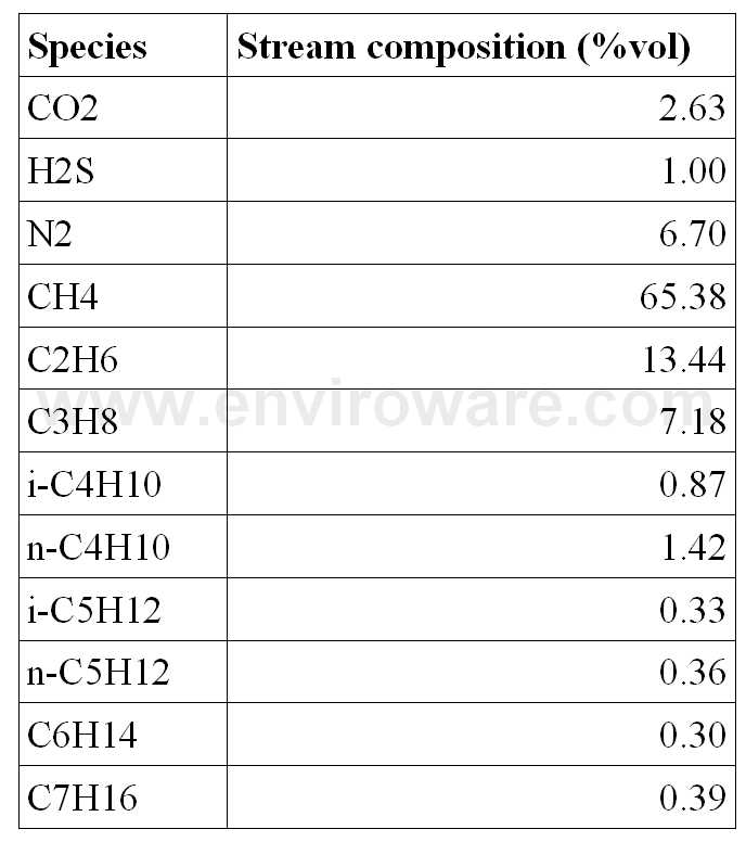
Table 1: Input stream composition (as in Alizadeh-Attar et al., 2007).
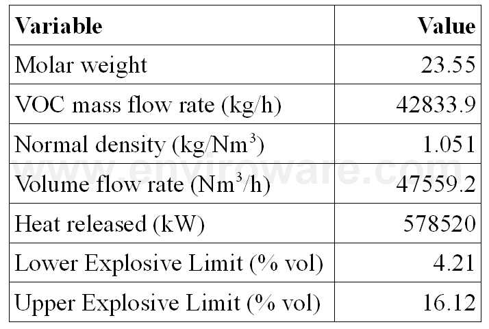
Table 2: Output stream composition.
The flue gas parameters calculated for the stream composition reported in Table 1, are reported in Table 3. The SO2 concentration and emission rate are calculated starting from the sulphur content in the fuel assuming that all H2S is converted to SO2, while concentrations and rates of the other pollutants are calculated starting from the AP42 emission factors assuming a light smoking flare (for particulate). The VOC emissions can alternatively be calculated by specifying a destruction efficiency as a software input.
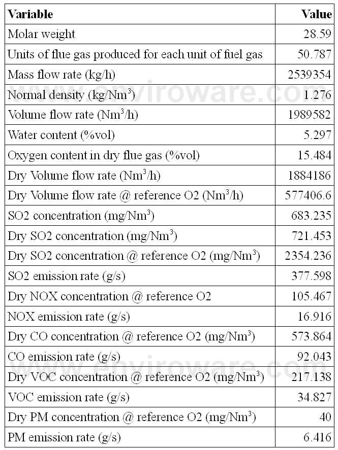
Table 3: Flue gas parameters.
The effective stack parameters needed for calculating the atmospheric dispersion of the pollutants emitted by the flare are calculated using an exit temperature of 1273 K, an exit speed of 20 m/s and an average ambient temperature of 293 K. Moreover, for the SCREEN3 EPA methodology a radiating heat loss equal to 55% is considered, while for the TCEQ methodology such value is calculated by the software as explained by Tan (1967). The calculated effective stack parameters are reported in Table 4. If the SCREEN3 methodology is used, the effective stack height to be specified within the dispersion model is the actual stack height plus the additional geometrical height (which represents the flame length).
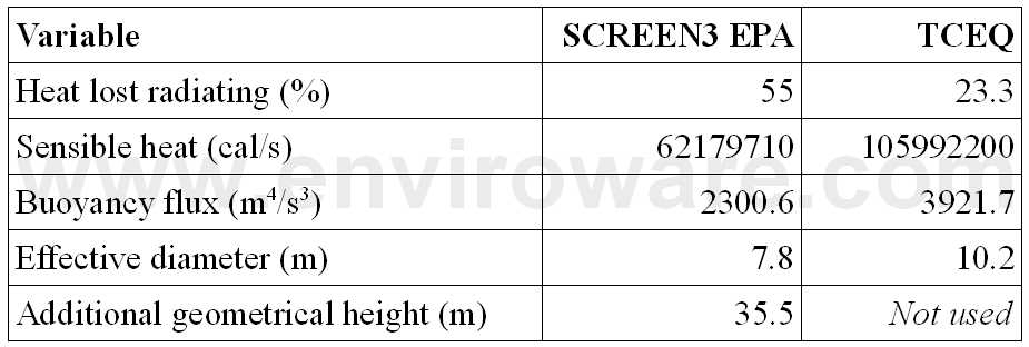
Table 4: Effective stack parameters to be used in atmospheric dispersion models.
The two different methodologies for calculating effective diameter and height will reflect on different air quality values when used within atmospheric dispersion models. As an example, the atmospheric concentration values have been calculated using both the methodologies with the TOXFLAM (Bianconi and Tamponi, 1993) analytical dispersion model, assuming a physical stack height of 20 m. The release of a generic pollutant with a rate of 1 g/s lasting for 10 minutes has been assumed. Figure 2 shows the time trend of the instantaneous concentrations estimated with the parameters indicated in Table 4 at a downwind distance of 500 m (wind speed 2 m/s, mixing height 1000 m, air temperature 293 K, stability class B), and 1000 m (wind speed 5 m/s, mixing height 1200 m, air temperature 293 K, stability class D). It is observed that the elevated values are due to the fact that they are instantaneous concentrations, not hourly concentrations. In fact, the hourly concentration calculated for example at 500 m downwind is 27.1 �g/m3with the EPA-SCREEN3 methodology, and 29.1 �g/m3 with the TCEQ methodology. Figure 3 shows the maximum instantaneous concentrations calculated at different downwind distances from the flare with the two methodologies. It is observed that, due to the lower emission height, the TCEQ methodology gives always greater concentrations.
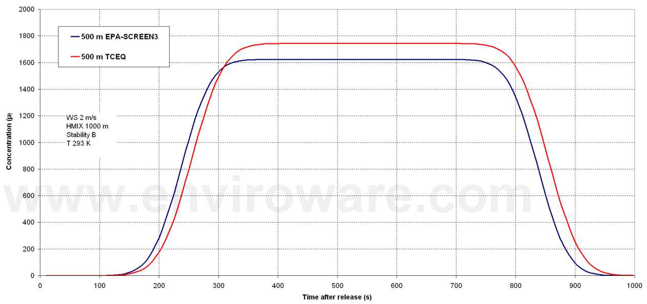
Figure 2a: Instantaneous concentrations calculated at 500 m and with two different meteorological conditions.
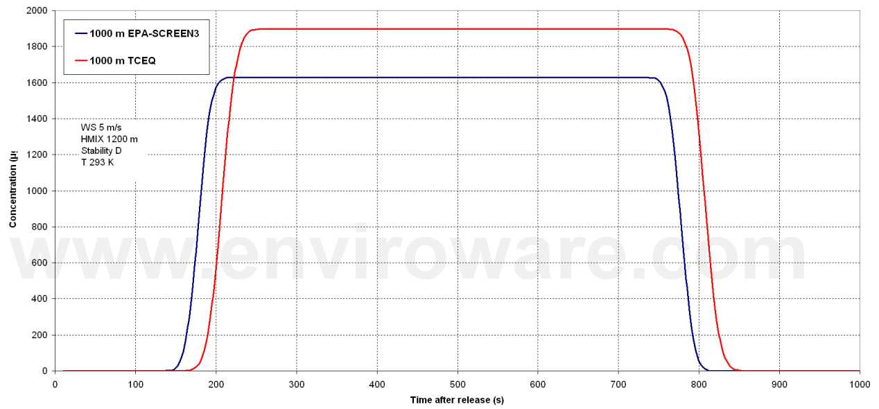
Figure 2b: Instantaneous concentrations calculated at 1000 and with two different meteorological conditions.
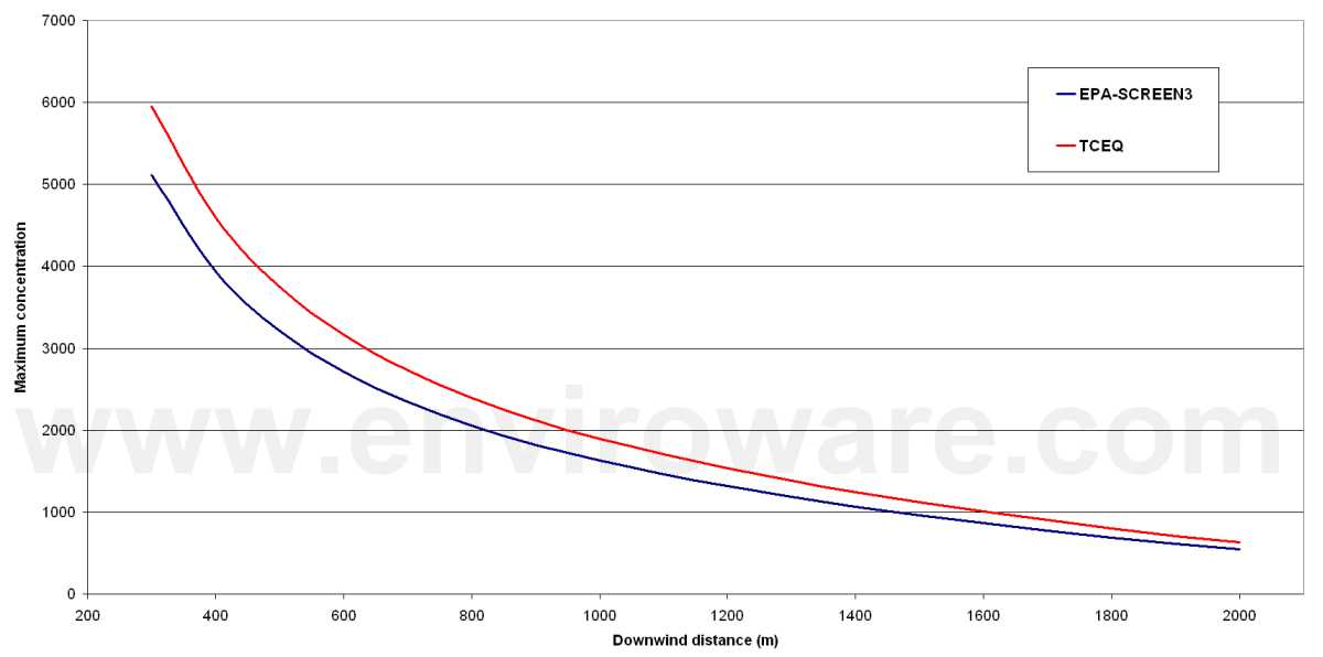
Figure 3: Maximum instantaneous concentrations calculated at different distances (wind speed 5 m/s, temperature 293 K, mixing height 1200 m, stability class D).
Stack sizing
A flare must be located so that it does not present a hazard to surrounding personnel and facilities, moreover for safety reasons a stack is used to elevate it. The height of the stack is determined based on the ground level limitations of thermal radiation intensity. If high surrounding structures are present close to the flare, the limiting thermal radiation may be calculated above the ground at a specific height. In this paragraph the stack diameter and height are calculated by specifying a maximum allowable thermal radiation value at ground at a specific horizontal distance from the stack basis (i.e. point B in Figure 1). The stream parameters calculated in the previous paragraph will be used as input values.
The allowable thermal radiation must be chosen accordingly to the user needs and the plant features. In this example a value of 6.3 kW/m2 will be used, which represents the maximum radiant heat intensity in areas where emergency actions lasting up to 30 s can be required by personnel without shielding but with appropriate clothing (which means hard hat, long sleeved shirts, work gloves, long legged pants and work shoes). The decision to consider in the calculation the contribution of the solar radiation depends mostly on the value of the allowable radiation. The maximum values of solar radiation span, approximately, the interval (0.8 � 1.0) kW/m2, depending on the position on the Earth and the period of the year. If the allowable radiation is relatively higher as the one indicated above, the inclusion of the solar radiation does not vary significatively the stack height (and then the costs).
On the contrary, for smaller values of the allowable radiation, the solar radiation must be considered because it has a high influence on the stack height. For example, for a continuous flare an allowable radiation of 1.58 kW/m2 (which is the maximum radiant heat intensity at any location where personnel with appropriate clothing can be continuously exposed) could be specified, which is almost comparable to the maximum solar radiation.
The flare stack height for different design wind speeds (from 6 m/s to 20 m/s) has been calculated using the stream composition illustrated in the previous paragraph. The input values used are summarised in Table5. The stack height has been calculated both with the simple methodology and with the B&S methodology. The stack diameter does not depend on the wind speed, therefore the two methodologies give always the same result of 0.33 m. On the contrary, the suggested stack height for different design wind speeds and for the two methodologies is illustrated in Figure 4. The suggested stack height is smaller when the B&S method is used.
Once the stack has been sized, it can be exported in Google Earth in the exact place where it is (or will be), as a vertical cylinder with correct height and diameter. An example is available here.
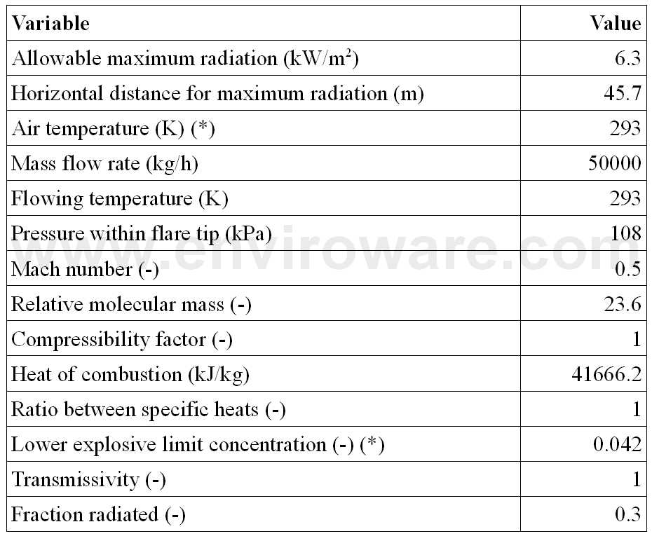
Table 5: Input values used for dimensioning the flare stack.
(*) The air temperature and the lower explosive limit concentration are needed only for the B&S method.
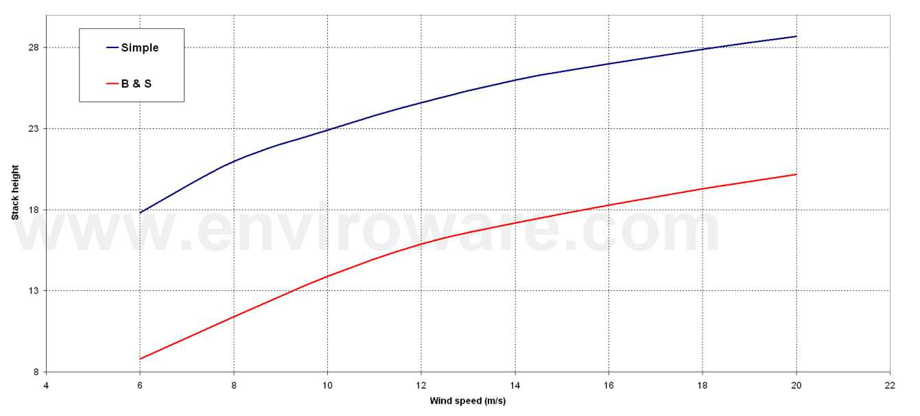
Figure 4: Stack height calculated for different design wind speeds and with the two methodologies (simple and B&S).
It is observed that the B&S method describes the flame tilting, and then the location of the flame centre, better than the simple method. However, the flame tilting with the B&S method must be calculated starting from non-dimensional parameters which contain the wind speed at denominator. This means that the B&S method cannot be used in completely calms conditions. Up to now it is not a big problem of course, because in calm conditions the flame is not tilted. Anyway, the tilting is graphically calculated (by means of curves digitised within FLARES), and the curves are defined only for some values of the adimensional parameters. This means that there will be some conditions which define the minimum and maximum values of the wind speed for the applicability of the B&S method. Defining the parameters A and B as follows
`A = (M_A) / (M_G C_L U_G)` `B = U_G D ((T_A M_G) / T_G)^(1/2)`where `M_A` is the air molar weight, `M_G` is the gas molar weight, `C_L` is the lower explosive limit (expressed as a fraction), `U_G` is the gas exit speed (m/s), D is the flare stack diameter (m), `T_A` is the air temperature (K) and `T_G` is the gas temperature (K), the more stringent of the two following conditions must hold:
`A/10 lt U_A lt 100/A` `B/1200 lt U_A lt B/3`Considering the values used in this paragraph, where the gas exit speed is 160.8 m/s, the last expression determines the most stringent conditions. The result is that in this case the wind speed must be greater than 0.22 m/s and smaller than 86 m/s; while the maximum wind speed is always respected, the minimum allowable wind speed must be checked. In some cases the minimum wind speed can be close to 1 m/s.
Thermal and acoustic impacts
As written in a previous section, beside atmospheric pollutants, when a flare operates, it generates heat radiation and noise.
In the following it will be considered a flare with a stack 22.9 m high, the input gas stream described in Table 1, and a wind speed of 10 m/s. The simple method will be used for the flame tilting. The parameters calculated by FLARES are a power liberated of 578697 kW, a flame length of 52 m, and an exit speed of 171 m/s.
Figure 5 shows the thermal radiation at ground as function of the horizontal distance from the flare stack. The values are shown for a constant unit transmissivity, and for transmissivities calculated for three values of the relative humidity: 40%, 60% and 80%. As shown, the transmissivity decreases increasing the relative humidity and the distance from the emitting point (the flame centre), therefore greater values are calculated for lower relative humidities. The maximum value of the thermal radiation is predicted in all cases for a point at about 15 m from the stack base, it is equal to about 10 kW/m2 for the case with unit transmissivity, while it is 1.7 kW/m2 less for the case with a relative humidity of 40%. The difference between the maximum thermal radiation predicted for a relative humidity of 40% and the one predicted for 80% is 0.3 kW/m2, and it decreases when the distance from the flame centre increases.
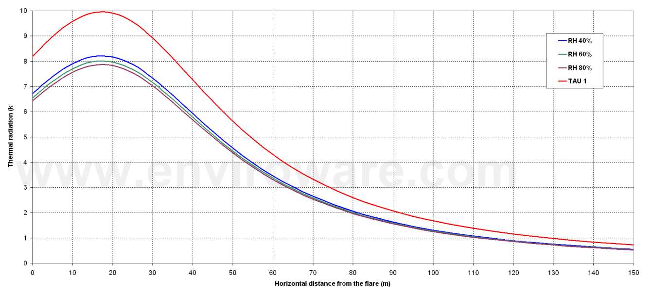
Figure 5: Thermal radiation at ground as function of the horizontal distance from the flare stack.
For the same stack, and using some of the input parameters shown in Table 5, the noise level at ground as function of the horizontal distance from the flare stack has been calculated (Figure 6). A pressure ratio of 2 has been used. With these input data FLARES calculates a speed of sound within the flared gas equal to 321.7 m/s, and a noise level at 30 m from the stack tip equal to 98.6 dB. The software keeps such noise level constant for distances smalled than 30 m from the stack tip (it is observed that Figure 6 is plotted against the horizontal distance from the stack base, not against the absolute distance from the stack tip), then it decreases according to the logarithm of the distance.

Figure 6: Noise at ground as function of the horizontal distance from the flare stack.
Maps of thermal radiation and acoustic levels can be exported in Google Earth. An example is available here for the thermal radiation.
Conclusions
Flaring is a unavoidable process in the production of oil and gas. A certain quantity of the gas needs to be flared at the production site for reasons of safety. Other times part of the gas produced with the oil is flared for reasons that may be a combination of geography and availability of customers. Flaring is also used in other types of industries, not only oil and gas. For these reasons it is important to have reliable methodologies and software tools which allow to evaluate the environmental impacts of the flaring activity: thermal radiation, noise and air pollution. Moreover, to guarantee the safety of operators and industrial structures and equipments, it is important to design stacks with correct heights and diameters according to the quantity of the flaring gas, its properties and the meteorological conditions (wind speed) of the site. The FLARES software, based on the API 521 Standards, is capable to carry out all these activities. Moreover it calculates the properties of the fuel gas and the flue gas starting from the molar composition of the fuel gas. This document presents some theoretical aspect of the software, describes its features and presents some examples of application.
References
- Alizadeh-Attar A., Ghoohestani H.R., Nasr Isfahani I. (2007) Reducing flare emissions from chemical plants and refineries through the application of fuzzy control system. Proceedings of the 6th WSEAS International Conference on Applied Computer Science, Hangzhou, China, April 15 17, 2007.
- API Standard 521 Pressure-relieving and Depressuring Systems, FIFTH EDITION, JANUARY 2007.
- Bader A., Baukal C.E. Jr and Bussman (2011) Selecting the proper flares systems. Chemical Engineering Progress (AIChE). pp. 45-50. http://www.aiche.org/cep/
- Bianconi R. and M. Tamponi (1993) A mathematical model of diffusion from a steady source of short duration in a finite mixing layer. Atmospheric Environment, 27A, 781-792.
- Briggs G.A. (1969) Plume Rise, USAEC Critical Review Series.
- Brzustowski T.A. and Sommer E.C. Jr. (1973) Predicting Radiant Heating from Flares. Proceedings Division of Refining, API 1973, Vol. 53, API Washington, D. C., p. 865-893.
- EPA (1995) SCREEN3 Model Users Guide. EPA-454/B-95-004. Pages 60.
- Hong J., Baukal C., Schwartz R and Fleifil M. (2006) Industrial scale flare testing. Chemical Engineering Progress (AIChE). pp. 35-39. http://www.aiche.org/cep/
- Obia A.E., Okon H.E., Ekum S.A., Eyo-Ita1 E.E., Ekpeni E.A. (2011) The Influence of Gas Flare Particulates and Rainfall on the Corrosion of Galvanized Steel Roofs in the Niger Delta, Nigeria. Journal of Environmental Protection, 2011, 2, 1341-1346.
- Tan S. H. (1967) Flare System Design Simplified. Hydrocarbon Processing, Vol. 46, No. 1, 172 176.
- TCEQ (2004) http://www.tceq.texas.gov/assets/public/permitting/air/memos/flareparameters.pdf
Read more and try FLARES for free